Mantel-Haenszel OR
Explanations & examples: Calculating the Mantel-Haenszel Odds Ratio is another way of detecting and adjusting for an eventual confounder by
stratification (by dividing the original, crude data into strata = "layers") similar to the approach under
Stratified Analysis only with slightly different calculations. If a variable is
suspected to be either an effect modifier or a confounder for a connection between an exposure and an outcome, then the original
2 × 2 table over the exposure and outcome can be stratified into two or more strata, each of the strata having a different
level of the potential confounding variable.
Calculating the Mantel-Haenszel Odds Ratio is another way of detecting and adjusting for an eventual confounder by
stratification (by dividing the original, crude data into strata = "layers") similar to the approach under
Stratified Analysis only with slightly different calculations. If a variable is
suspected to be either an effect modifier or a confounder for a connection between an exposure and an outcome, then the original
2 × 2 table over the exposure and outcome can be stratified into two or more strata, each of the strata having a different
level of the potential confounding variable.Input types: If you already have the data in 2 × 2 tables, you should choose the default input type "2 × 2 tables". If, on the other hand, you have the data as data in a text file, then you should choose input type "raw data". Furthermore; if the data in your text file is in the following format:  then you should also click the check option "data in file is in columns" to the right before copy/pasting into the table or reading from a data file. If the data in your text file is in the following format; 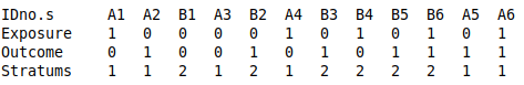 Then you should instead click the check mark "data in file is in rows" to the right before copy/pasting or reading from a data file. Example:In this fictive, made-up example we investigate whether alcohol consumption could be an effect modifier or confounder for the connection between hypertension and stroke. We start with the original "crude" 2 × 2 table over the exposure (hypertension) and outcome variables (stroke) without any stratification:  As can be seen, the OR (Odds Ratio) value for this crude table is 1.9554 meaning that those who had hypertension have a 1.9554 times higher odds of getting the outcome (stroke) than those who didn't have hypertension. The connection is significant on a 5 % significance level since the OR value is significantly different from 1 (the number 1 is not included in the 95 % confidence interval [1.0532 : 3.6304], which starts above 1 and ends above 1). We now stratify this crude table into 2 strata after different levels of alcohol consumption to see if the variable "alcohol consumption" is either an effect modifier or a confounder for the connection between hypertension and getting a stroke. In the first strata are the persons with little or no alcohol consumption, in the second the ones with regular alcohol consumption. 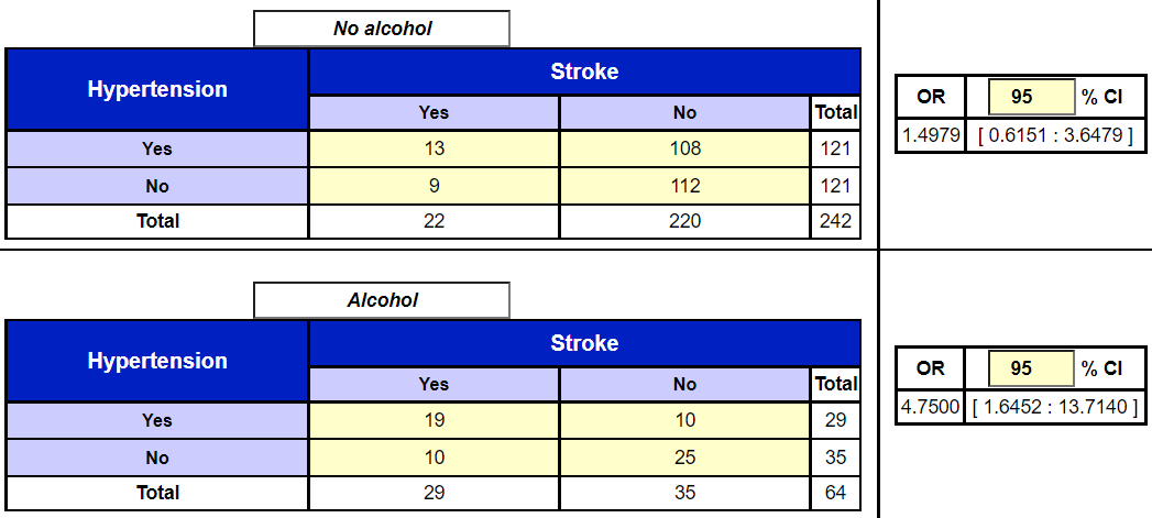 First it is checked whether the two OR values from the strata could be assumed equal. This is done by performing a chi-squared test of homogeneity:  As seen, the p-value is 0.1023 and therefore slightly above 0.05 so we cannot reject the null hypothesis H0 claiming that the two OR values of 1.4979 and 4.75 could be the same. So the two OR values are not significantly different from each other on a 5 % significance level. And therefore the variable stratified after (alcohol consumption) is not an effect modifier. If p < 0.05 alcohol consumption would, in fact, have been an effect modifier for the connection between hypertension and stroke, because the effect that hypertension has on stroke would then be different (would be modified) depending on the alcohol consumption. And we would then have stopped here and proceeded no further (since something can not be both an effect modifier and a confounder at the same time). Knowing that alcohol consumption is not an effect modifier for the connection between hypertension and stroke, we proceed to check for confounding by calculating the Mantel-Haenszel weighted estimate of the odds ratios from the 2 strata:  The Mantel-Haenszel weighted estimate of OR = 2.4087 deviates noticably from the crude OR value of 1.9554. As a rule of thumb, the difference between the crude OR and the Mantel-Haenszel weighted OR must be 20 % or more to consider the variable stratified after to be a confounder. This is the case here, so it seems like alcohol consumption could be a confounder for the connection between having hypertension and getting a stroke. The "rule of five" at the bottom of the page is a mechanism to check the validity of the Mantel-Haenszel chi-square-test. Both "totals" of the Min and Max columns have to differ from the total of the expected values by 5 or more for the test to be valid. More info and formulas under the page Formulas. In order to establish with certainty if alcohol consumption is really a confounder we look at the confounder triangle and the criteria for something to be a confounder:  The criteria for something to be a confounder (C):
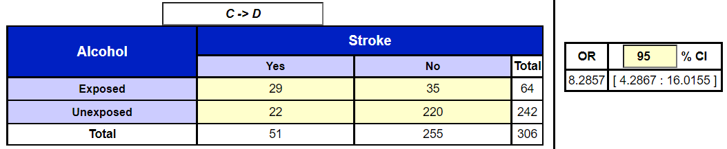 The table has been created by adding the cells together vertically in each of the strata (in other words using the 4 "totals" of the columns in the strata tables). The OR value of this table is then OR = 8.2857 and is significantly different from 1 (since 1 is not included in the 95 % confidence interval of the OR [4.2867 : 16.0155]). So there is a connection between the possible confounder and the outcome and the arrow C → D is established. Finally, the last criterion (the double arrow between E and C) has to be checked in order for the confounder to be fully established. This can be done with the following 2 × 2 table: 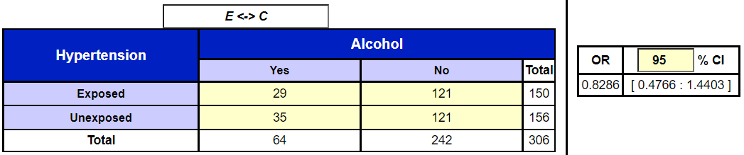 Also here the table was created by combining strata 1 and 2 into one table over alcohol consumption vs. hypertension by adding the cells in the strata tables horizontivally (using the "totals" of the rows). As can be seen the OR value for this table is 0.8286. This OR value is not significant on a 5 % significance level, because 1 is included in the 95 % confidence interval going from 0.4766 to 1.4403. So it seemed at first glance that alcohol consumption could be a confounder for the connection between hypertension and stroke by comparing the Mantel-Haenszel weighted OR with the crude OR, but the last arrow between E and C in the confounder triangle could not be established. And since all 3 criteria have to be fulfilled for something to be a confounder, the conclusion is that alcohol consumption is neither an effect modifier nor a confounder for the connection between hypertension and stroke in this fictive, made-up example. If alcohol consumption had in fact been a confounder, then the Mantel-Haenszel weighted estimate of the OR values would have been the "true" impact that hypertension has on stroke after having adjusted for the confounding effect of alcohol consumption. Meaning that people with hypertension would have had a 2.4087 times higher odds of getting a stroke compared with people with no hypertension, adjusted for alcohol consumption. |
|
No. of strata:
|
Decimals:
|
|||||
|
|
|||||||||||||||||||||||||||||||
|
|
|||||||||||||||||||||||||||||||