Data Analysis
Explanations & examples: If the data in your text file looks like this:
 Then you should choose the option "data in file is in columns" to the right when copy/pasting or uploading. If, on the other hand, the data in your text file looks like this:  Then you should choose the option "data in file is in rows" to the right when copy/pasting or uploading. Concepts in data analysisClick "Calculate" to perform the data analysis on all the data sets. In the section "results" are the calculated values of the concepts in data analysis; mean value, variance, standard deviation, prediction interval of the mean, confidence interval of the mean, skewness, kurtosis, minimum, maximum. There are two versions of the variance (var) and of the standard deviation (SD). If the data set involved is only a sample (part) taken from a population, then the version Var(sample) and SD(sample) should be chosen. If the data set involved is the entire population, then the versions Var(population) and SD(population) should be chosen. There are some small differences in the formulas for the calculations whether it's a sample or a population. See under "means" in the page with the formulas. Skewness and kurtosis are concepts to check whether data sets could be assumed normally distributed. The skewness of a data set should be 0 or close to 0 in order for it to be normally distributed (because the bell shaped normal distribution has a skewness of 0; it is not skewed, but rather symmetrical around the mean). The kurtosis should be 3 or close to 3 for the data set to be assumed normally distributed. For more info and formulas, see the page with the formulasZ-Test, F-Test and T-Test between two data setsBoth a z-test and a t-test can be performed on any two of the involved data sets to test whether their mean values could be assumed equal (mean1 = mean2 or conversely mean1 - mean2 = 0). Just select the data sets to be tested in the drop-down selector boxes "Data Set "1" versus Data Set "2" ". A t-test is more precise, because it involves the data sizes (the no. of values in the data sets) contrary to a z-test. But the t-test is also more cumbersome, because it's first necessary to do an f-test to see whether the two variances in the data sets involved could be equal. If the p-value in the f-test is more than 0.05 (p > 0.05) then we cannot reject the null hypothesis H0 that the two variances could be the same. In this case we proceed with the t-test version "assuming equal variance" and the common variance (SD2) is being calculated together with the common SD. Otherwise, if p < 0.05 we reject the H0 on a 5% significance level that the two variances of the data sets could be the same (i.e. that their ratio is 1) and therefore choose the t-test version "assuming different variances". The difference in the p-values of the two t-test versions is usually not very large. If the p-value in the t-test is below 5% (p < 0.05) then we reject on a 5% significance level that the null hypothesis that the two data sets could have the same mean (we reject that the mean difference could be zero). In this case the confidence interval of the mean difference (MD) will not contain 0. If p > 0.05 in the t-test then we don't reject H0 and the two means could be equal (MD could be 0). In this case the confidence interval of the MD will contain 0 (go from a negative number to a positive number). Same procedure if a z-test is chosen instead; also here the p-value (p < 0.05 or p > 0.05) determine whether we can reject or not reject the null hypothesis of equal means (MD = 0).In this example, we perform tests on the data sets no. 1 and 3: 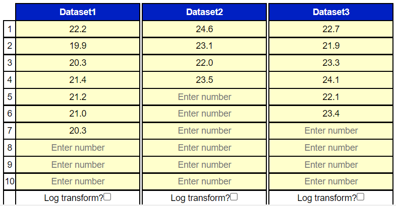 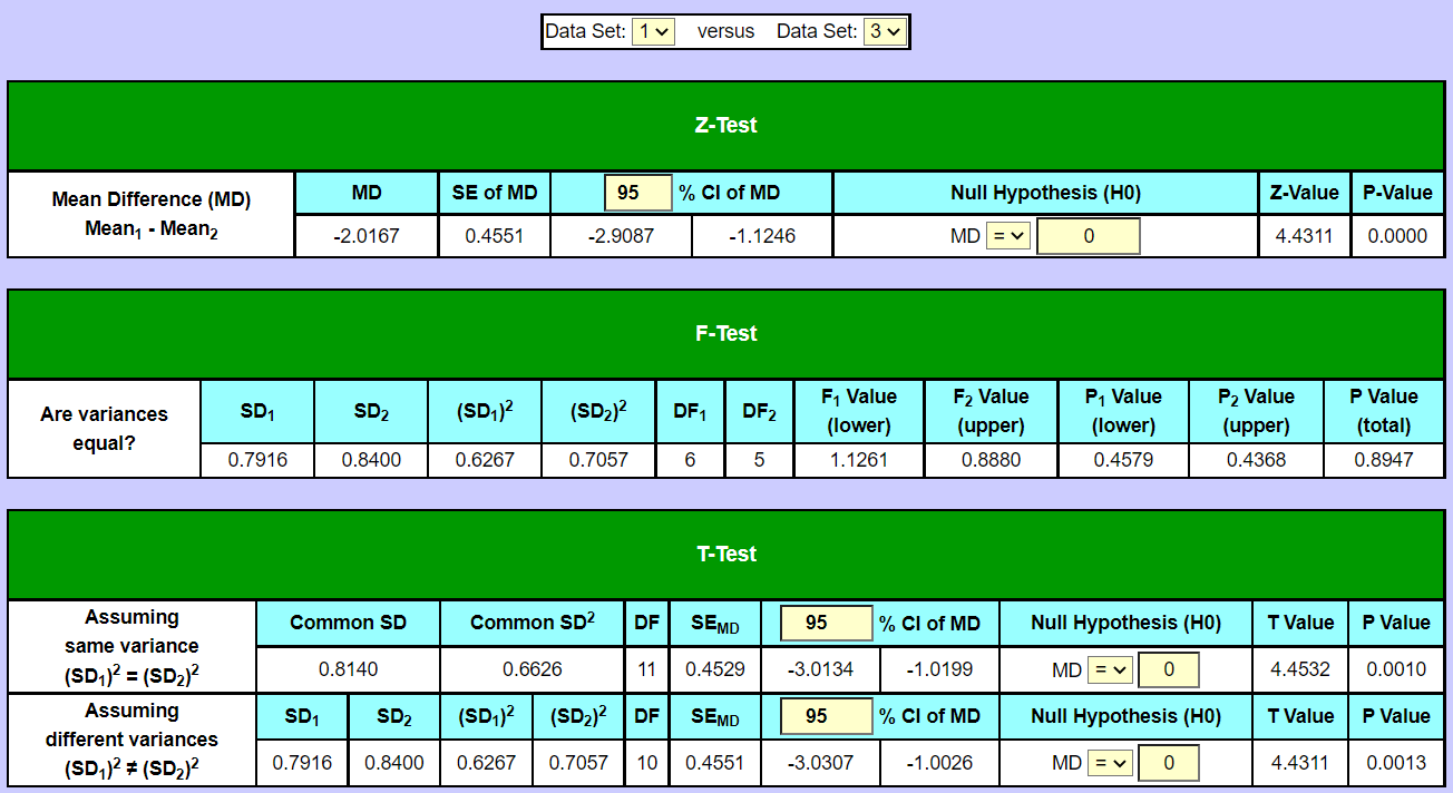 Here, the p-value in the f-test is 0.8947 which is above 0.05, therefore we don't reject the null hypothesis, that the variances of the two data sets could be equal. We therefore choose the t-test version "assuming same variance", which gives a t-value of 4.4532 and a p- value of 0.001. Since the p-value is below 0.05 we reject the null hypothesis here that the mean values could be the same, therefore the two means are significantly different from each other (and their difference, MD, significantly different from 0). This can also be seen in that 0 is not included in the span of the 95% confidence interval of the mean difference [-3.0134 : -1.0199]. Also note that the confidence intervals of the two means (in section "results") are [20.3136 : 21.4864] and [22.2445 : 23.5888] respectively, so the intervals don't overlap each other, which they also shouldn't do since the means are different. And the means are not included in each other's confidence interval. Instead of an f-test and a t-test a z-test could also have been chosen. Here, the z-value is 4.4311 and the p-value is 0.0000, which is (of course) far below 0.05. Note: If the confident intervals of the two mean values in question don't overlap at all, then it isn't really necessary to do a test, because in this case we know the mean values are significantly different from each other and we know beforehand that the p-value will be under 0.05. If one of the mean values lies within the the confidence interval of the other mean value (or if both mean values lies within each other's confidence intervals), then it also isn't necessary to do a test, because then we know that the two mean values could be equal and that the p value will be over 0.05. If there is some overlap between the two confidence intervals, but neither of the two means is included in the other one's confidence interval, then the result is uncertain by looking at the confidence intervals alone and it is necessary to do a test (either z-test or t-test). ANOVA (Analysis Of Variance)There are two versions of ANOVA, the two-way-ANOVA and the one-way-ANOVA. A prerequisite for performing the two-way-ANOVA is that there is the same no. of values (entries) in the data sets involved. If not, only the one-way-ANOVA can be performed. In the two-way-ANOVA both the variations between the data sets (columns) is being investigated as well as the variations between the rows. To see if there is significant variation between the data sets (columns) involved, the mean value for each data set is calculated and those mean values are then compared by looking at their distances to the overall mean. The overall mean is the average of all the data values from all the data sets involved. If the F-value here is too large (and the p value therefore under 0.05) then the means of the data sets differ too much on average from the overall mean to say that there's no significant variation between the columns. To see if there's significant variation between the rows, the mean value for each row (across data sets) is calculated and all of these mean values then compared with the overall mean by looking at their deviations from it. If the deviations are too large on average then the variations between the rows are too big to say that there's no statistical significant variation between the rows (p < 0.05).Example:11 patients are having their systolic blood pressure measured 3 times on a single day. Morning, noon and evening. That gives the following data sets: Important detail here is that it is (of course) the exact same 11 patients measured again, only at different times. Also the order of the patients in the data sets must be preserved. The questions are now: Does the time of measure have an effect on the blood pressure (is there difference between the columns). And: Is there significant variation between the 11 patients in the study? Both p-values are below 0.05 so the time of the day has (in this made up example) had an effect on the blood pressure. And the 11 patients (the rows) differ significantly from each other in terms of blood pressure.  In the one-way-ANOVA, on the other hand, it cannot be assumed that the data sets have tha same number of inputs (entries), although they of course can have that. In the one-way-ANOVA we look at the mean value of each data set and compare it to the overall mean of all the values. And then we look at the distances from each value in the data sets to the mean of its own data set. If the data values in the data sets on average deviates more from their respective data set's mean value than the mean values of the data sets deviate from the overall mean, then the variation for the data sets involved is to large to be ignored as non-significant and the p-value is below 0.05. For more info on ANOVA, please see the page formulas Graphs and PlotsIn section graphs &plots it's possible to do some data visualization over the data sets in the input table. A boxplot can be drawn over one single data set or over all involved data sets, same goes for violin plot and scatter plot (point plot). A histogram can be drawn over a single data set to see whether it can be assumed to be normally distributed. If so, the histogram is approximately bell shaped like the curve of the Gaussian bell curve (the normal distribution probability density function). Another way of checking normality is to make a QQ-plot (a normal quantile plot), where the z-values of the standard normal distribution are compared to the values of the data set in question. The points will approximately lie on a stright line, if the data set is normally distributed. An XY-plot can be drawn between two data sets with one data set along the x-axis and the other along the y-axis to see if there's a linear connection between the two data sets. This requires that the data sets have the same no. of values.To select more than one variable, hold down ctrl (or cmd) when clicking in the drop down selector box.  |
No. of data sets: |
No. of rows: |
Decimals:
|
|||||||||||||||||||||||||||||||||||||||
|
||||||||||||||||||||||||||||||||||||||||||